Strain fitting of 2D data in GSAS-II
For this tutorial, data were collected with a MAR2300 area detector at APS 1-ID-C with a wavelength 0.12398 Å (100mm diameter beam) from a 1.5mm square hot rolled steel test specimen; the front surface has been dusted with some CeO2 to aid in calibration. Three images are used here; one is with no load on the sample and the other two are with the sample under tension along the y-axis (vertical). The loading will distort the steel (ferrite & austenite) diffraction rings and our purpose here is to characterize this distortion via a strain model by B. B. He & K. L. Smith (Adv. in X-ray Anal. 41, 501, 1997). Note that menu entries are listed in bold face below as Help/About GSAS-II, which lists first the name of the menu (here Help) and second the name of the entry in the menu (here About GSAS-II).
Step 1: Start GSAS-II and read the images
Use the Data/Read image data menu item to
read the data file into a new GSAS-II project. A file selection dialog will be
shown; its appearance will depend on your OS. Change the search directory to 2Dstrain/data and then select the files nx09_strain_001.mar2300, nx09_strain_006.mar2300 and
nx09_strain_011.mar2300
and press Open. Select the 1st
image (001) from the GSAS-II data tree and select Image Controls; adjust the Max intensity so that the CeO2 rings are visible (~1500 will
suffice or 99%). You should see:
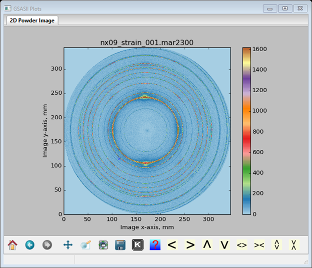
For the image and
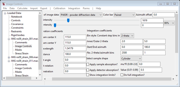
for the controls.
Step 2: Calibration of the detector position
This image is a superposition of three diffraction patterns; CeO2 calibrant, ferrite (BCC iron) and austenite (FCC iron). Consequently the calibration needs to be done with some care; the steps are as follows:
Set the wavelength to 0.12398
Set the calibrant to CeO2 SRM674b
Set Min calib d-spacing to 1.09; this avoids picking a CeO2 ring that overlaps one of the steel ones.
Pick Show ring picks? check box
Set Pixel search range to 5; the rings are fairly widely separated will little chance for overlap.
Use Calibration/Calibrate, select 5 points on the inner CeO2 ring with left mouse button and start calibration with right mouse button. The result should be something like
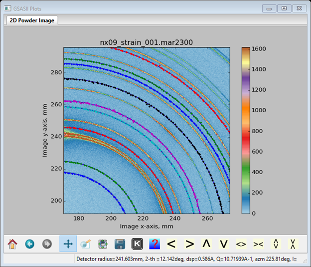
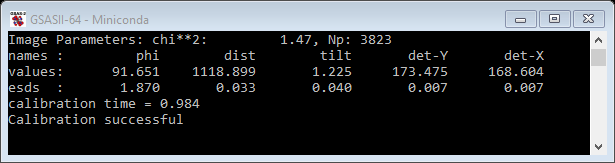
I’ve zoomed in to show that the CeO2 rings are well fitted and don’t overlap any of the more intense steel ones. The calibration results show on the data window
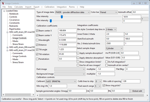
and the console
You should now copy these results to the other images. Use Parms/Copy controls; a popup dialog will appear; select Set All and OK.
Step 3: Fitting unstrained steel
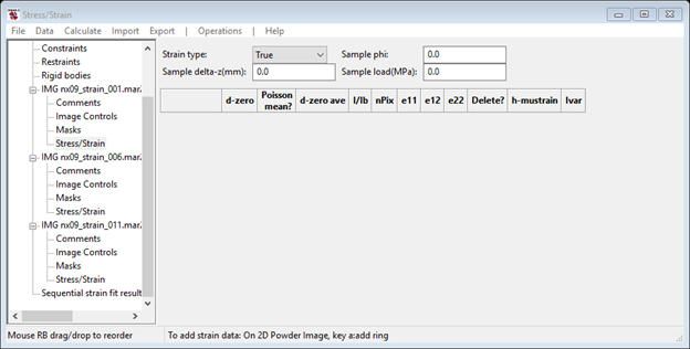
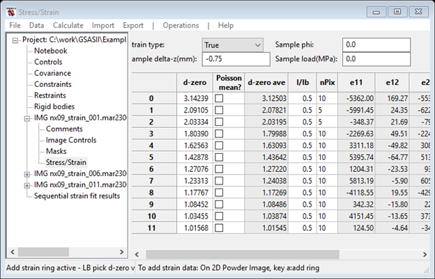
In this step you will select the diffraction rings to be analyzed for strain; it is best to pick a few CeO2 ones as well to confirm that the sample position does not shift during loading. Select the first image (001) and the Stress/Strain tree item. An empty plot (“Strain”) will appear and the initial Stress/Strain data window
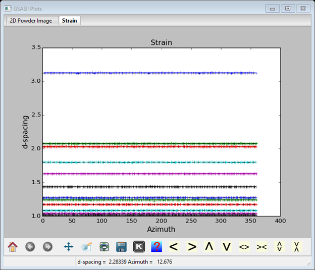
Change Sample delta-z to -0.75 since center of the steel sample is that much closer to the detector than the CeO2 calibrant. Then select 2D Powder Image and follow the instruction to add a ring; press a and use the mouse left button to select a ring. Do as many as you like but be sure to select some CeO2 rings as well; it is useful to zoom in to help with the selection, but make sure zoom buttons are off for the selection. You can control the image display with the Image Controls. Each time you pick a ring, GSAS-II show the 2D Powder Image zoomed in where you were looking before your selection. I chose 12 rings. Do Operations/Fit stress/strain; the Strain plot is updated to show
Notice that each ring is plotted in different colors (they may be somewhat mixed for the two lines ~2Å! We will fix this next). The 2D Powder Image shows the picks as well

And the rings are listed on the Stress/Strain data window; a scroll bar allows easy access to all the entries.
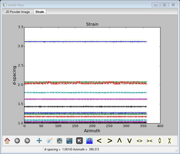
If necessary, we can now fix the mixing of the two 2Å lines; change the Pixel search range to 5 for both. Do Operations/Fit Stress Strain. After you are done the Strain plot should look like
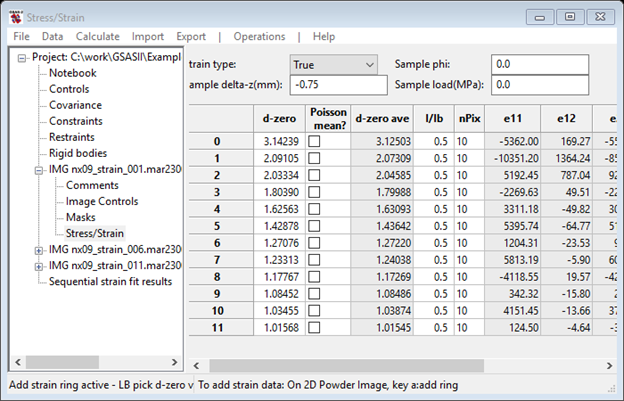
We are now ready for the first strain fit; do Operations/Fit stress/strain. Each ring will be fitted to the three strain tensor elements (ε11, ε12 & ε22) that can be determined from a single 2D diffraction ring. The resulting Strain plot now shows curves calculated from the fitted tensor elements; these are very nearly straight lines as expected from an unloaded sample. In particular the austenite 111 line (~2.08Å) is much flatter than the ferrite 200 line (~2.03Å); this reflects the sample history (hot rolled steel). The tensor elements with esds are shown on the console and in the data window
The d-zero ave is the average d-spacing around each ring; this can be used as the reference d-spacing. If Poisson ave is checked then d-zero ave is determined from
If e11
< e22: d-zero ave = dmin-(dmax-dmin)/4;
else: d-zero ave = dmin+3*(dmax-dmin)
Where dmin,dmax are the minimum and maximum d-spacings for a given diffraction ring, thus selecting the place where the diffraction ring under load would give a strain free value.
Each d-zero value for this no load sample can be set to this value; this will suppress any residual stress offset. To update all the d-zero values to the calculated ones do Operations/Update d-zero then repeat Operations/Fit stress/strain. Repeat as needed to make d-zero match d-zero ave for all lines so that h-mustrain (= d-zero/d-zero ave -1) is small (less than ~±250). I got for the no load sample
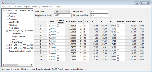
Ivar is the variance in the normalized ring intensity; if >0 the sample is textured in some way. Finally you want this set of d-zero values to be applied to the images from the loaded sample; do Operations/Copy stress/strain to apply them to the other images.
Step 4: Sequential fitting of steel under load
For the result of the sequential fitting to make sense, we need to enter the applied load for each image. Unfortunately, this must be done by hand here because the load value is not in the image header. The loads are: 001: - 2.17425, 006: 527.917 and 011: 1004.41 all in newtons (N). Each needs to be divided by the cross section area (2.25mm2) of the sample; GSAS-II will do this bit of math for you, and this gives the values in MPa. For image 001 enter -2.17425/2.25 in the Sample load (MPa) box, 527.917/2.25 for image 006 and 1004.41/2.25 for image 011. When done the data window for image 011 should look like
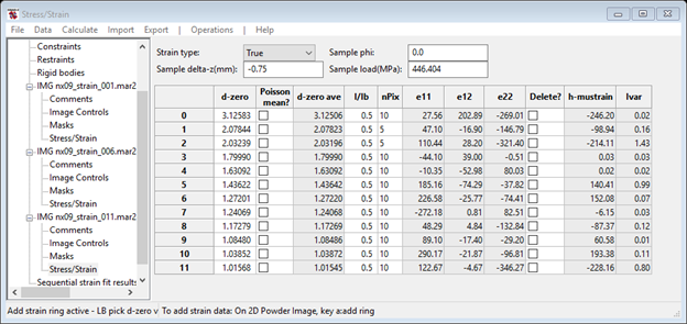
Note that if the beam line software has prepared the appropriate file containing this information, it could be loaded via the Operations/Load sample data menu item.
Next, we do the sequential refinement. Do Operations/All image fit from the Stress/Strain data window menu from any of the images. A popup window will show the selection of images
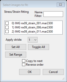
Press Set All, all
boxes will be checked showing selection of the data sets. This also allows you
to instruct the sequential refinement to start at the last data set and proceed
backwards through them (Reverse order). It also allows you
to instruct the sequential refinement to use the current parameters as starting
values for the next data set. This works in either direction and facilitates
the initial sequential refinements. Select just Copy to next and press
OK;
the sequential refinement will proceed very rapidly displaying results for each
data set on the console and finally ending by displaying the Sequential strain
fit result.
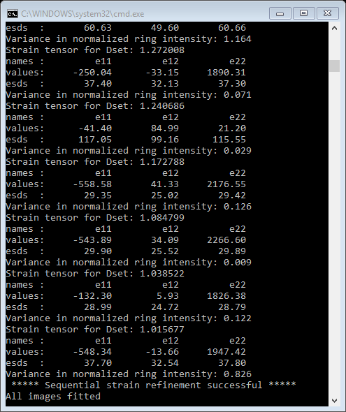
I only show the bottom of the listing. The data window shows the results of the sequential fit.
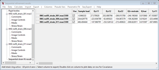
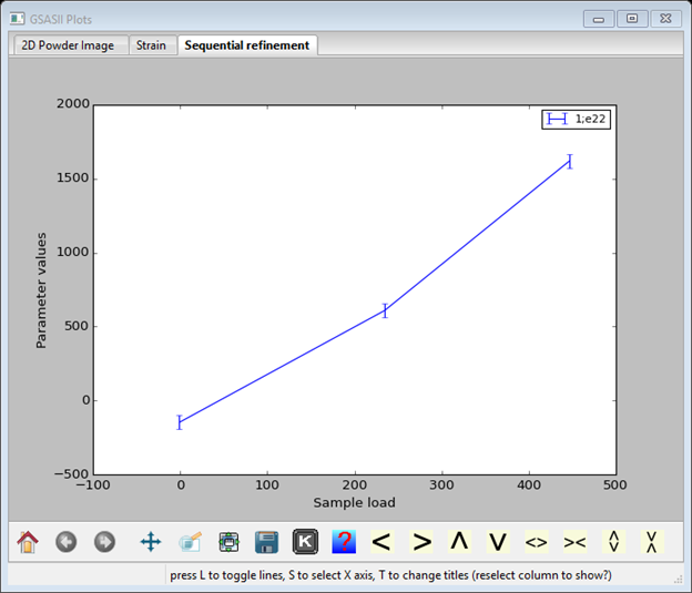
This table is the results of the sequential fit to the three images. There are columns for each parameter. If you double click on a column heading (try a steel e11 or e22 – I selected 1;e22 from my list). The plot shows the variation of this parameter with image sequence; press ‘s’ and select Sample load and the plot will show (you’ll have to pick something else & then back to 1:e22).
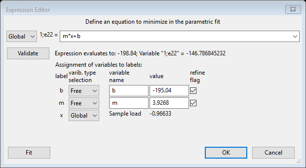
We can next fit this to a straight line. Select Parametric fit/Add equation, select a variable (Global) in the 1st pull down box (I chose 1;e22) and enter m*x+b in the equation box; the frame will change to give selections for m, x & b. Use Free for m & b and Global/Sample load (at the bottom of list) for x. Then press Fit. The Expression Editor window should look like; press OK to exit this window.
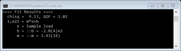
And the console shows the parameters with esds
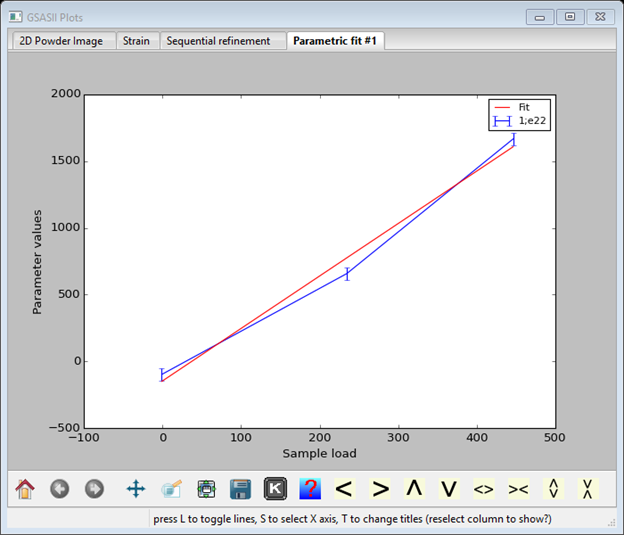
The plot will show the best fit line
You can explore other features of this facility; pick more than one column (single click on the label) and the Selected cols/Plot selected menu item to plot them together.
To see the effect of stress on one diffraction line, select the Strain plot and zoom in on one line (I zoomed in on just one line; ferrite 211) from image 011.
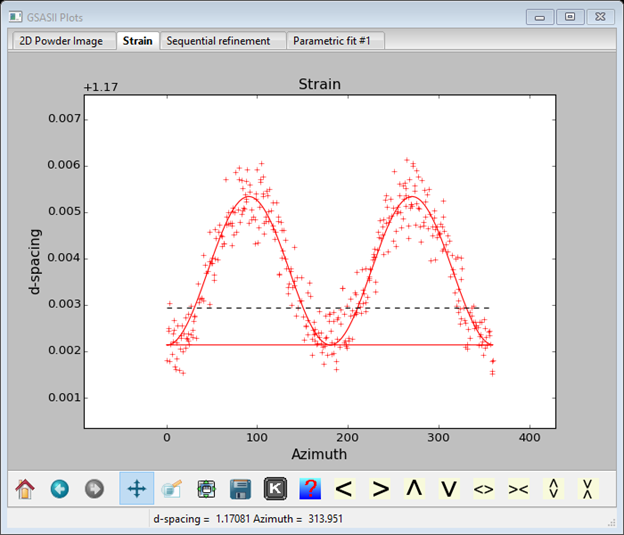
The dashed line gives the d-zero position. When you look at the other lines, you should notice that the ones at ca. 3.13Å, 1.63Å, and 1.24Å remain straight lines; these are from CeO2 and should be unchanged under load.
Finally we can investigate the appearance of texture in the ring intensities, do Operations/Plot intensity distribution. A new plot appears; the ‘u’ key will change the curve offsets to get
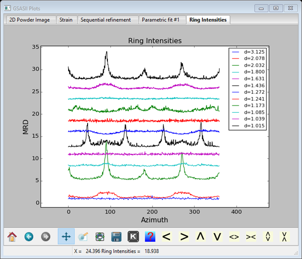
The CeO2 lines are straight (MRD=1.0) while lines from the two steel phases show the effect of texture but little graininess.
Again you could save the project with File/Save project on the main GSAS-II data tree menu although it is not needed for any further tutorials. The strain results from each image can be exported as a comma delimited set of values which can easily be read by Microsoft Excel and other spread sheet programs; see Export/Image data as/Strain CSV file.